
Optimizing Databricks Performance: Liquid Clustering and Deletion Vectors in Practice

Introduction
Teams running Databricks in production face the classic triangle: performance, cost, and operational effort. Traditional tuning approaches like partitioning strategies, periodic OPTIMIZE, ZORDER BY, cluster sizing, and shuffle tuning still work – but they require continuous rework as data volumes grow and query patterns change.
Databricks keeps pushing Delta Lake performance forward. While Photon has been around for years (it became the default for newly created Databricks SQL endpoints back in 2021), two features are particularly relevant for most modern lakehouse projects:
Liquid Clustering is a modern data layout optimization that replaces manual partitioning and ZORDER, allowing your layout to evolve without full rewrites.
Deletion Vectors (DV) provide „soft-delete“ metadata that helps avoid rewriting entire Parquet files for row-level changes and powers faster updates on Photon-enabled compute.
What Problems do Liquid Clustering and Deletion Vectors Solve?
In practice, these features address different challenges:
- Slow selective reads: Filters scan too many files or row groups
- Expensive updates, deletes, and merges: Small changes rewrite large files
Liquid Clustering mainly targets problem (1), while Deletion Vectors target problem (2) – and you’ll often use both together.
Feature Overview
Liquid Clustering (LC)
Liquid Clustering organizes data based on clustering keys and improves data skipping for filters on those keys. It’s designed to replace partitioning and ZORDER, and it’s not compatible with them. Liquid Clustering is generally available for Delta tables with Databricks Runtime 15.2+ and can be used for all new tables, including streaming tables and materialized views.
How it works: Liquid Clustering groups related data physically on storage so selective queries scan fewer files. Unlike static partitioning, clustering keys can be adjusted later without completely rewriting the existing data structure [1].
Deletion Vector (DV)
Deletion Vectors store row-level changes as metadata (deleted or updated rows) rather than immediately rewriting every affected data file. Databricks uses DV to power Predictive I/O for updates on Photon-enabled compute.
The principle: Instead of rewriting the entire Parquet file when you DELETE, UPDATE, or MERGE a row, DV marks the row as modified. The current table state is then resolved during reads by applying modifications from the deletion vector.
Important: Enabling DV upgrades the table protocol, so older clients may not be able to read the table [2].
Photon
Photon is Databricks native vectorized query engine for faster SQL and DataFrame execution. While not „new,“ it’s critical because several modern optimizations (like Predictive I/O on Azure Databricks) are explicitly Photon-based.
Note: Predictive I/O is Databricks‘ umbrella term for Photon-only runtime optimizations that make data interactions faster. It covers (1) accelerated reads, which speed up scanning and filtering, and (2) accelerated updates, which reduce full file rewrites for DELETE, UPDATE, and MERGE by leveraging Deletion Vectors on supported Photon-enabled compute.
Hands-on Lab: Liquid Clustering and Deletion Vectors in Practice
Prerequisites
- Workspace with DBR 15.2+ available
- Photon-enabled compute option:
- Databricks SQL Warehouse (Photon typically enabled), or
- Cluster with Photon enabled
Creating Schema and Dataset
First, let’s create a demo schema and generate a reproducible dataset with PySpark. The dataset simulates a fact table with:
- High-cardinality customer_id
- Time filtering on event_date
- Numeric amount value
CREATE SCHEMA IF NOT EXISTS performance_demo;
USE performance_demo;
from pyspark.sql import SparkSession
from pyspark.sql.functions import col, rand, expr, date_add, lit
from datetime import datetime, timedelta
# Generate dataset
spark.range(0, 200_000_000) \
.withColumn("customer_id", (rand() * 100_000).cast("int")) \
.withColumn("event_date",
date_add(lit(datetime(2024, 1, 1)), (rand() * 365).cast("int"))) \
.withColumn("amount", (rand() * 1000).cast("decimal(10,2)")) \
.write.format("delta").mode("overwrite") \
.saveAsTable("sales_unclustered")
Liquid Clustering in Practice
What is Liquid Clustering and When Should You Use It?
Liquid Clustering replaces partitioning and ZORDER and allows you to redefine clustering keys without completely rewriting the existing data layout. It’s explicitly not compatible with partitioning or ZORDER.
Databricks enables LC via the CLUSTER BY (...) clause:
CREATE TABLE sales_lc
CLUSTER BY (customer_id, event_date)
AS SELECT * FROM sales_unclustered;
Triggering Clustering with OPTIMIZE
Liquid Clustering is incremental and typically applied via OPTIMIZE:
OPTIMIZE sales_unclustered;
OPTIMIZE sales_lc;Running a Selective Query and Comparing Query Performance
Let’s choose a realistic predicate (high-cardinality customer + narrow date range):
SELECT SUM(amount) AS total_amount
FROM sales_unclustered
WHERE customer_id = 12345
  AND event_date BETWEEN '2024-06-01' AND '2024-06-30';

SELECT SUM(amount) AS total_amount
FROM sales_lc
WHERE customer_id = 12345
  AND event_date BETWEEN '2024-06-01' AND '2024-06-30';
The same query on sales_unclustered vs. sales_lc shows clear differences:
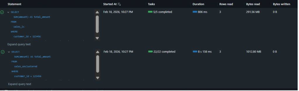
sales_unclustered and sales_lc.| Metric | sales_unclustered | sales_lc (Liquid Clustering) |
|---|---|---|
| Wall-clock Duration | 8 s 158 ms | 806 ms |
| % of bytes pruned during scan | 0% | 88% |
| Bytes read | 1,020 MB | 291 MB |
| Rows read | 3 | 3 |
| Files read | 12 | 2 |
| % of files pruned during scan | 0% | 82% |
Observation: Liquid Clustering didn’t just reduce runtime – it dramatically accelerated query performance by over 10x (from 8.2 seconds down to 806 milliseconds). This improvement stems directly from aggressive data pruning: 88% of bytes and 82% of files were skipped during the scan phase. The query scanned only 291 MB across 2 files instead of 1,020 MB across 12 files, demonstrating exactly the behavior you want for selective predicates with high-cardinality filters like customer_id combined with date ranges. The same 3 rows were returned, but with a fraction of the I/O cost.
Deletion Vectors in Practice
What Are Deletion Vectors?
Deletion Vectors record row-level changes as metadata and apply them physically later during rewrite or maintenance operations (e.g., OPTIMIZE).
Creating Two Identical Tables: DV Off vs. DV On
To enable DV, we set the Delta property delta.enableDeletionVectors:
-- DV OFF
CREATE TABLE dv_off
AS SELECT * FROM sales_unclustered
LIMIT 200_000_000;

-- DV ON
CREATE TABLE dv_on
TBLPROPERTIES ('delta.enableDeletionVectors' = 'true')
AS SELECT * FROM sales_unclustered
LIMIT 200_000_000;Compacting Tables before Testing
OPTIMIZE dv_off;
OPTIMIZE dv_on;Running a Small DELETE and Comparing Query Performance
Let’s execute a small DELETE operation:
DELETE FROM dv_off
WHERE customer_id > 123456 AND event_date = '2024-01-07';

DELETE FROM dv_on
WHERE customer_id > 123456 AND event_date = '2024-01-07';
The operation metrics show clear differences:
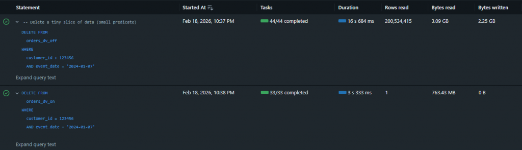
| Metric | dv_off (Deletion Vectors Off) | dv_on (Deletion Vectors On) |
| Total wall clock duration | 16 s 684 ms | 3 s 333 ms |
| Rows read | 200,534,415 | 1 |
| Bytes read | 3.09 GB | 763 MB |
| Bytes written | 2.25 GB | 0 |
| Files read | 24 | 12 |
| Files written | 24 | 0 |
| Rows written | 199,465,585 | 0 |
| Deletion vectors added | 0 | 1 |
Observation: With DV OFF, the delete operation took 16.7 seconds and required significant data rewriting (24 files written, 2.25 GB of data written, nearly 200 million rows rewritten). With DV ON, the same delete completed in just 3.3 seconds – approximately 5x faster – with zero files or bytes written. Instead of rewriting data files, Databricks recorded the deletion via a single deletion vector, avoiding the expensive rewrite operation entirely while still processing the deletion logic (evident in the 763 MB read for scanning).
Advantages and Limitations
Advantages
Liquid Clustering:
- Dynamic adaptation of data layout without full rewrites
- Significantly reduced I/O through improved data skipping
- Simplified maintenance compared to manual partitioning + ZORDER
- Compatible with streaming tables and materialized views
Deletion Vectors:
- Faster row-level changes since not every change forces immediate full-file rewrites
- Enables/boosts update acceleration features on Photon compute (Predictive I/O on Azure Databricks)
- Drastic reduction in bytes rewritten for DELETE/UPDATE/MERGE operations
Limitations
Liquid Clustering:
- Not compatible with traditional partitioning or ZORDER
- Requires DBR 15.2+ for production use
- Initial setup must carefully choose clustering keys (though they can be adjusted later)
Deletion Vectors:
- Enabling DV upgrades table protocol – older clients or applications may not be able to read the table
- Manifest generation limitations exist when DV is present (requires purge first –
REORG TABLE ... APPLY (PURGE)) - Platform-specific restrictions can apply
Note: A manifest generation workflow is the process used to make Delta tables readable by query engines that don’t understand Delta’s transaction log.
Conclusion
Liquid Clustering and Deletion Vectors are two powerful features in the Databricks platform that each address different performance challenges. Liquid Clustering optimizes selective reads through intelligent data layout, while Deletion Vectors accelerate expensive row-level operations.
For production environments, a combined strategy could be recommended: Liquid Clustering for frequently filtered columns and Deletion Vectors for tables with regular updates or deletes. The practical benchmarks show that both features deliver significant performance improvements – Liquid Clustering achieves up to 90% reduction in scanned data, while Deletion Vectors reduce rewrite time by over 80%.
The investment in properly configuring these features pays off long-term through lower costs, better performance, and reduced operational effort. With Databricks Runtime 15.2+, data engineering teams have a modern toolbox to elevate lakehouse performance to a new level.
References
[1] How Liquid Clustering Actually Works – Data Engineer Wiki